第十二讲-因子分析判别分析
习题10.3
1. 题目要求
2.解题过程
解:
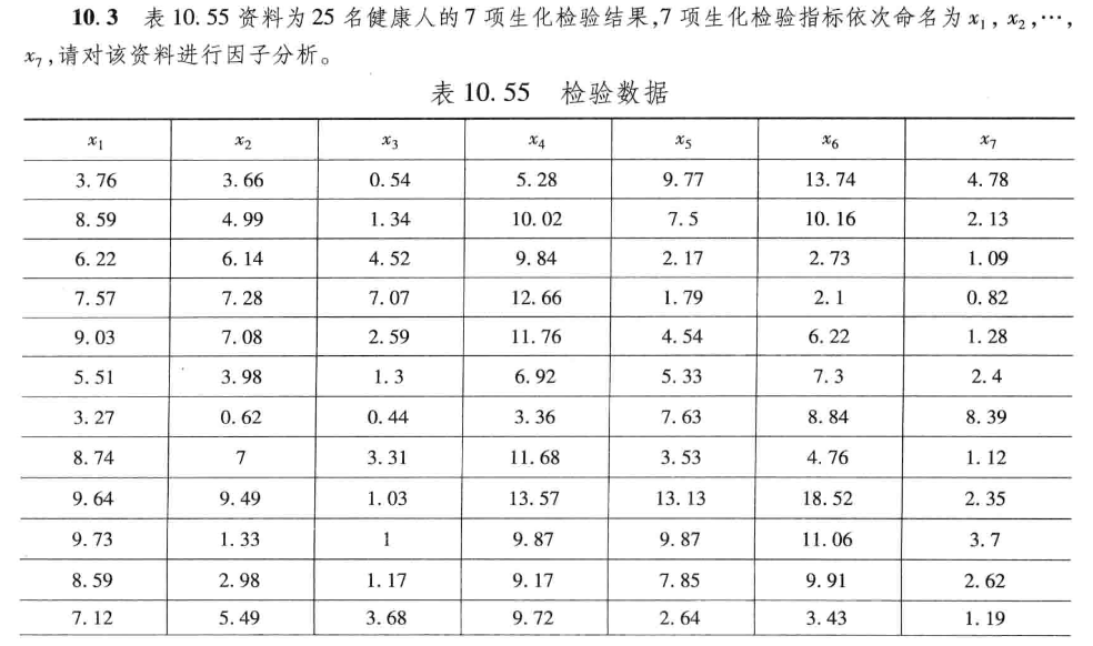
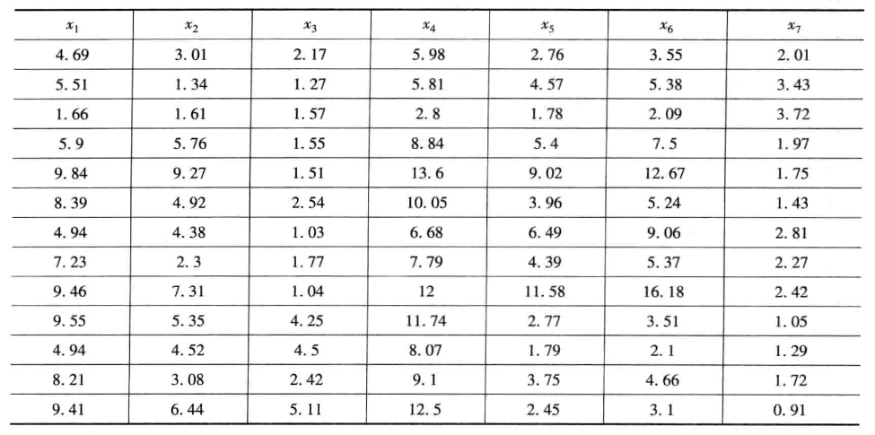
先将数据标准化,记第 \(i\) 个评价对象的第 \(j\) 个评价指标值为 \(a_{ij},i=1,2,...25;j=1,2,...7\) ,将 \(a_{ij}\) 标准化为 \(\widetilde{a}_{ij}\) : $$ \widetilde{a}{ij}=\frac{a{ij}-\mu_j}{s_j} $$ 式中: $$ \mu_j=\frac{1}{25}\sum_{i=1}^{25}a_{ij} $$
接下来计算相关系数矩阵 \(\mathbf{R}\) : $$ \mathbf{R}=(r_{ij})_{7\times7} $$
式中 \(r_{ii}=1,r_{ji}=r{ij},r_{ij}\) 是第 \(i\) 指标和第 \(j\) 指标的相关系数。
计算初等载荷矩阵,首先算出相关矩阵 \(\mathbf{R}\) 的特征值 \(\lambda_1\geq\lambda_2\geq...\geq\lambda_7\),以及应的特征向量\(\mathbf{u}_1,\mathbf{u}_2,...,\mathbf{u}_7\),则初等载荷矩阵为: $$ \mathbf{\Lambda}_1=[\sqrt{\lambda_1}\mathbf{u}_1,\sqrt{\lambda_1}\mathbf{u}_2,...,\sqrt{\lambda_1}\mathbf{u}_7] $$ 计算得出前三个特征值的贡献率达到了 \(98\%\) ,选择三个主因子,对提取的因子载荷矩阵进行旋转,得到矩阵 \(\mathbf{\Lambda}_2=\mathbf{\Lambda}^{(3)}_1\mathbf{T}\) ,
取\(\mathbf{\Lambda}_1\)的前三列,\(\mathbf{T}\)为正交矩阵,构造因子模型: $$ \begin{align} \begin{cases} \widetilde{x}1=\alpha{11}\widetilde{F}1+\alpha{12}\widetilde{F}2+\alpha{13}\widetilde{F}3 \ \vdots\ \widetilde{x}_7=\alpha{71}\widetilde{F}1+\alpha{72}\widetilde{F}2+\alpha{73}\widetilde{F}_3 \end{cases} \end{align} $$ 最终,得到了三个因子,第一个因子是 \(x_1\) ,第二个因子是 \(x_5\) ,第三个因子是 \(x_2\) 。
3.程序
求解的MATLAB程序如下:
clc, clear

% 给定的原始数据矩阵
dd = [3.76, 3.66, 0.54, 5.28, 9.77, 13.74, 4.78; ...
    8.59, 4.99, 1.34, 10.02, 7.5, 10.16, 2.13; ...
    6.22, 6.14, 4.52, 9.84, 2.17, 2.73, 1.09; ...
    7.57, 7.28, 7.07, 12.66, 1.79, 2.1, 0.82; ...
    9.03, 7.08, 2.59, 11.76, 4.54, 6.22, 1.28; ...
    5.51, 3.98, 1.3, 6.92, 5.33, 7.3, 2.4; ...
    3.27, 0.62, 0.44, 3.36, 7.63, 8.84, 8.39; ...
    8.74, 7, 3.31, 11.68, 3.53, 4.76, 1.12; ...
    9.64, 9.49, 1.03, 13.57, 13.13, 18.52, 2.35; ...
    9.73, 1.33, 1, 9.87, 9.87, 11.06, 3.7; ...
    8.59, 2.98, 1.17, 9.17, 7.85, 9.91, 2.62; ...
    7.12, 5.49, 3.68, 9.72, 2.64, 3.43, 1.19; ...
    4.69, 3.01, 2.17, 5.98, 2.76, 3.55, 2.01; ...
    5.51, 1.34, 1.27, 5.81, 4.57, 5.38, 3.43; ...
    1.66, 1.61, 1.57, 2.8, 1.78, 2.09, 3.72; ...
    5.9, 5.76, 1.55, 8.84, 5.4, 7.5, 1.97; ...
    9.84, 9.27, 1.51, 13.6, 9.02, 12.67, 1.75; ...
    8.39, 4.92, 2.54, 10.05, 3.96, 5.24, 1.43; ...
    4.94, 4.38, 1.03, 6.68, 6.49, 9.06, 2.81; ...
    7.23, 2.3, 1.77, 7.79, 4.39, 5.37, 2.27; ...
    9.46, 7.31, 1.04, 12, 11.58, 16.18, 2.42; ...
    9.55, 5.35, 4.25, 11.74, 2.77, 3.51, 1.05; ...
    4.94, 4.52, 4.5, 8.07, 1.79, 2.1, 1.29; ...
    8.21, 3.08, 2.42, 9.1, 3.75, 4.66, 1.72; ...
    9.41, 6.44, 5.11, 12.5, 2.45, 3.1, 0.91];

% 标准化数据(Z-score标准化)
stdd = zscore(dd);

% 计算标准化数据的相关系数矩阵
r = corrcoef(stdd);

% 使用PCA对相关系数矩阵进行主成分分析,获取特征向量(vec1)、特征值(val)和贡献率(con)
[vec1, val, con] = pcacov(r);

% 计算符号矩阵f1,其大小与vec1一致,元素值均为vec1所有元素的和的符号
f1 = repmat(sign(sum(vec1)), size(vec1, 1), 1);

% 将特征向量(vec1)与符号矩阵(f1)相乘,得到新的特征向量矩阵(vec2)
vec2 = vec1 .* f1;

% 计算矩阵f2,其大小与vec2一致,元素值均为val中的特征值的平方根
f2 = repmat(sqrt(val)', size(vec2, 1), 1);

% 将vec2与f2相乘,得到最终的载荷矩阵(a)
a = vec2 .* f2;

% 设定保留的主成分数目
num = 3;

% 保留前num个主成分
am = a(:, [1:num]);

% 使用varimax方法对主成分进行旋转,获得旋转后的载荷矩阵(b)以及得分矩阵(t)
[b, t] = rotatefactors(am, 'Method', 'varimax');

% 将未保留的主成分载荷也加入旋转后的载荷矩阵,得到旋转后的完整载荷矩阵(bt)
bt = [b, a(:, [num + 1:end])];

% 计算每个变量在各个主成分上的载荷的平方和,得到公共度(degree)
degree = sum(b.^2, 2);

% 计算每个主成分的总的贡献率(contr)
contr = sum(bt.^2);

% 计算被保留的主成分的累计贡献率(rate)
rate = contr(1:num) / sum(contr);

% 计算因子分析的系数矩阵(coef)
coef = inv(r) * b;
4.结果
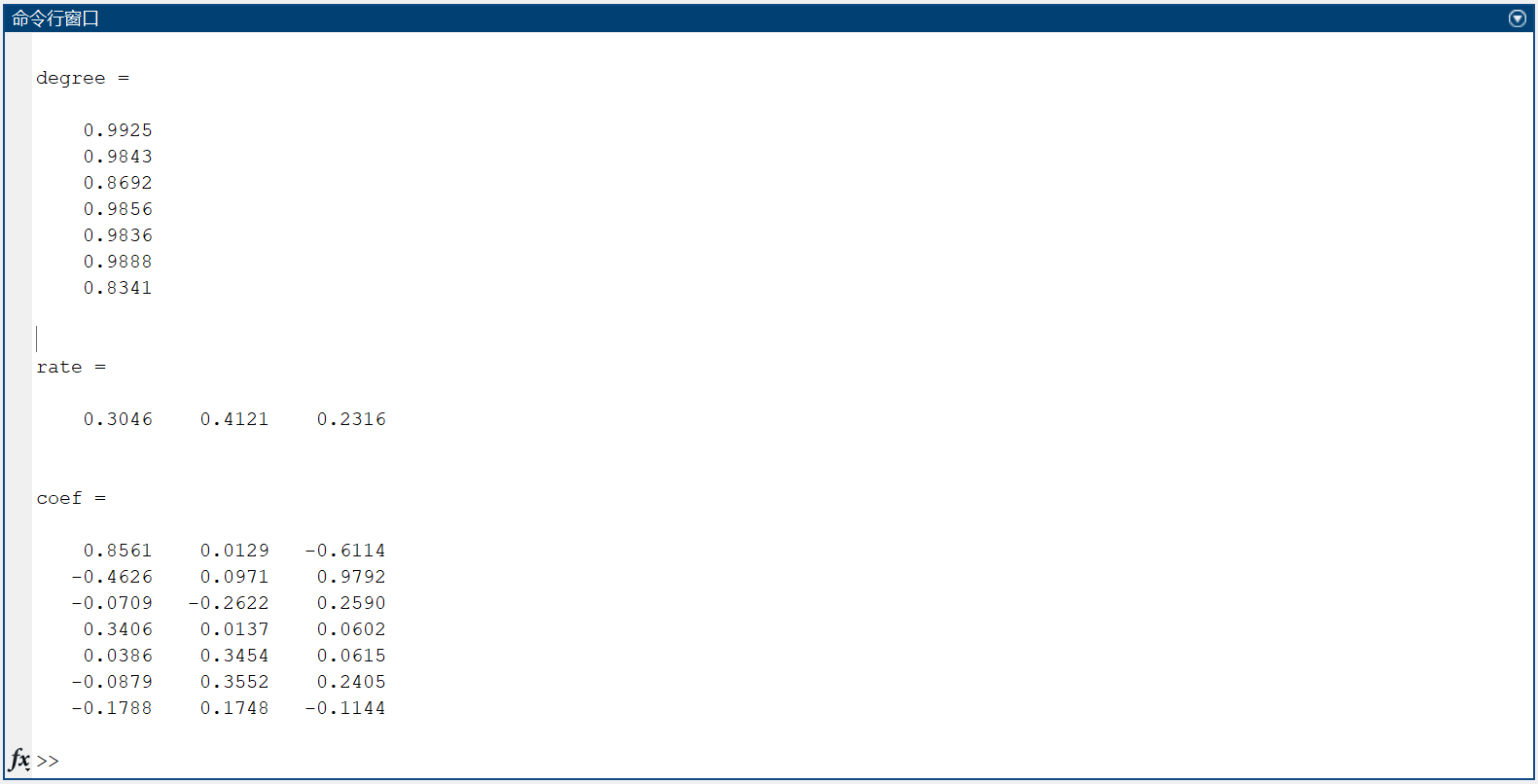
得到的因子分析表如下:
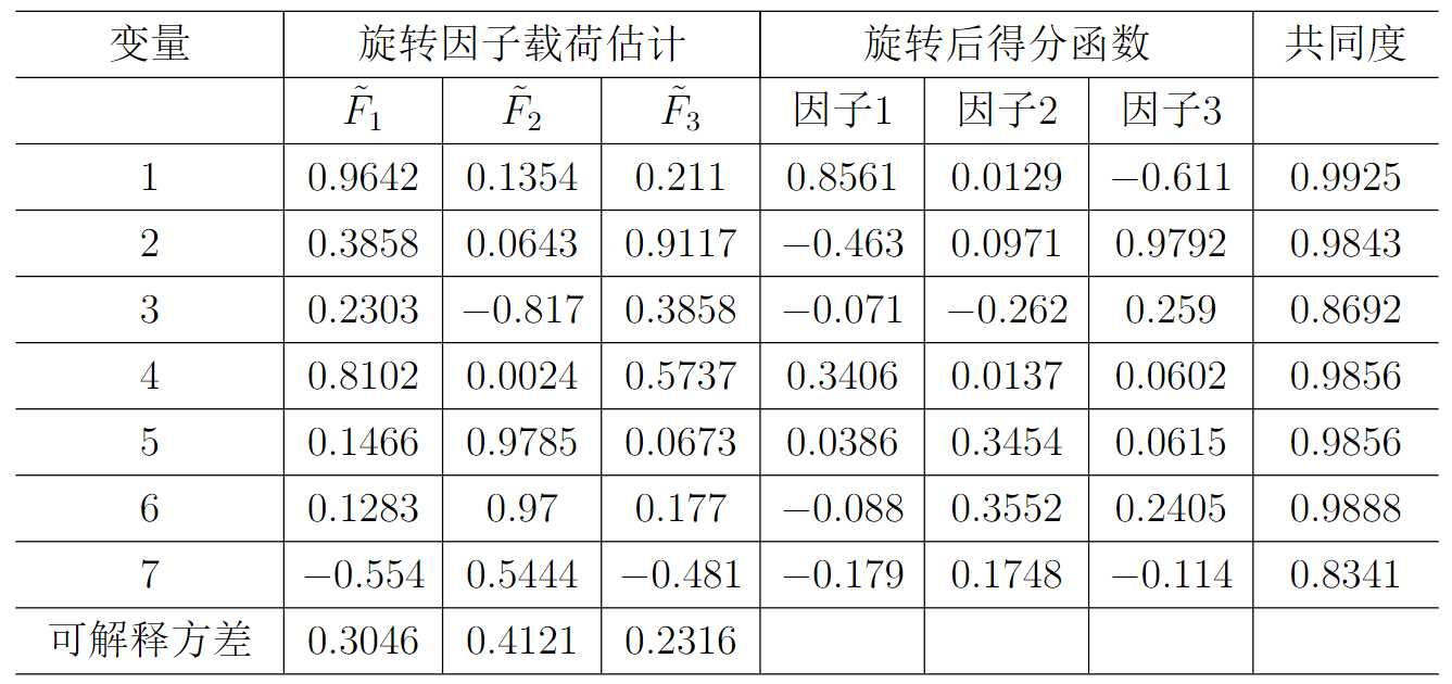
得到了三个因子,第一个因子是 \(x_1\) ,第二个因子是 \(x_5\) ,第三个因子是 \(x_2\) 。
习题10.6(1)
1. 题目要求

2.解题过程——对应分析
解:
分别用 \(i=1,\dots,16\) 表示,以 \(a_{ij}\) 表示第 i 个地区第 j 个指标变量 \(x_j\) 的取值。
记: $$ \mathbf{A}=(a_{ij}){16\times6} $$ 记: $$ a{i\cdot}=\sum_{j=1}^{6}a_{ij},a_{\cdot j}=\sum_{i=1}^{16}a_{ij} $$ 首先把 \(\mathbf{A}\) 化为规格化的“概率”矩阵 \(\mathbf{P}\) , 记 \(\mathbf{P}=(p_{ij})_{16\times6}\) ,其中 \(p_{ij}=a_{ij}/\mathbf{T}\) ,\(\mathbf{T}=\sum_{i=1}^{16}\sum_{j=1}^{6}a_{ij}\)。再对数据进行对应变换,令 \(\mathbf{B}=(b_{ij})_{16\times6}\) ,其中: $$ b_{ij}=\frac{p_{ij}-p_{i\cdot}p_{\cdot j}}{\sqrt{p_{i\cdot}p_{\cdot j}}}
= \frac{a_{ij}-a_{i\cdot}a_{\cdot j}/\mathbf{T}}{\sqrt{a_{i\cdot}a_{\cdot j}}},
i=1,2,\dots, 16,j=1,2,\dots,6. $$ 对 \(\mathbf{B}\) 进行奇异值分解,\(\mathbf{B}=\mathbf{U}\varLambda \mathbf{V}^{\mathbf{T}} (,其中 \(\mathbf{U}\) 为 \(16\times 16\) 正交矩阵,\)\mathbf{V}\)为 \(6\times6\) 正交矩阵,\(\varLambda =\begin{bmatrix} \varLambda_m &0\\ 0&0 \end{bmatrix}\),这里 $ \varLambda_m=diag(d_1,\dots,d_m) $ ,其中 \(d_i(i=1,2,\dots,m)\) 为 \(\mathbf{B}\) 的奇异值。
记 \(\mathbf{U}=[\mathbf{U_1} \vdots \mathbf{U_2}],\mathbf{V}=[\mathbf{V_1} \vdots \mathbf{V_2}]\) ,其中 \(\mathbf{U_1}\) 为\(16\times m\) 的列正交矩阵,\(\mathbf{V_1}\) 为 \(6\times m\) 的列正交矩阵,则 \(\mathbf{B}\) 的奇异值分解式等价于\(\mathbf{B}=\mathbf{U_1}\varLambda\mathbf{V_1}^T\)。
记 \(\mathbf{D_r}=diag(p_{1\cdot},p_{2\cdot},\dots,p_{16\cdot}),\mathbf{D_c}=diag(p_{\cdot1},p_{\cdot2},\dots,p_{\cdot6})\) ,其中 \(p_{i\cdot}=\sum_{j=1}^{6}p_{ij}\) ,\(p_{\cdot j}=\sum_{i=1}^{16}p_{ij}\)。则列轮廓的坐标为 \(\mathbf{F}=\mathbf{D}_{c}^{-1/2}\mathbf{V_1}\varLambda_m\) ,行轮廓的坐标为 \(\mathbf{G}=\mathbf{D}_{r}^{-1/2}\mathbf{V_1}\varLambda_m\) 。最后通过贡献率的比较确定需要截取的维数,形成对应分析图。
计算 \(\mathbf{B^T}\mathbf{B}\) 的特征值,惯量,表示相应维数对各类别的解释量,最大维数 \(m=\min{16-1,6-1}\) ,本例最多可以产生5个维数。从下表可看出,第一维数的解释量达 77.4% ,前两个维数的解释度已达92.1%。
| 维数 | 奇异值 | 惯量 | 贡献率 | 累积贡献率 |
|---|---|---|---|---|
| 1 | 0.189893 | 0.036059 | 0.773764 | 0.773764 |
| 2 | 0.082831 | 0.006861 | 0.147224 | 0.920988 |
| 3 | 0.047138 | 0.002222 | 0.047618 | 0.968669 |
| 4 | 0.03113 | 0.000969 | 0.020795 | 0.989464 |
| 5 | 0.022159 | 0.000491 | 0.010536 | 1 |
行坐标
| 北京 | 天津 | 河北 | 山西 | 内蒙古 | 辽宁 | |
|---|---|---|---|---|---|---|
| 第一维 | -0.07905 | -0.06783 | -0.26354 | 0.457766 | 0.07715 | -0.13567 |
| 第二维 | -0.0354 | 0.138818 | -0.10045 | -0.05715 | 0.156316 | -0.08455 |
| 吉林 | 黑龙江 | 上海 | 江苏 | 浙江 | 安徽 | |
|---|---|---|---|---|---|---|
| 第一维 | -0.27126 | -0.19757 | 0.386809 | 0.086955 | 0.079122 | -0.14212 |
| 第二维 | -0.00074 | 0.045985 | -0.07833 | -0.04222 | -0.01969 | -0.14225 |
| 福建 | 江西 | 山东 | 河南 | |
|---|---|---|---|---|
| 第一维 | -0.17469 | -0.18859 | 0.069823 | -0.1462 |
| 第二维 | -0.11317 | -0.1527 | 0.100318 | 0.032858 |
列坐标
| x1 | x2 | x3 | x4 | x5 | x6 | |
|---|---|---|---|---|---|---|
| 第一维 | -0.07905 | -0.06783 | -0.26354 | 0.457766 | 0.07715 | -0.13567 |
| 第二维 | -0.0354 | 0.138818 | -0.10045 | -0.05715 | 0.156316 | -0.08455 |
在下图中,给出16个地区和6个指标在相同坐标系上绘制的散布图。

从图中可以看出,地区和指标点可以分为两类,
第一类包括指标点 \(x_4,x_5\) ,地区点为北京、天津、河北、上海、江苏、浙江、山东;
第二类包括指标点 \(x_1,x_2,x_3,x_6\) ,地区点为其余地区。
3.程序
求解的MATLAB程序如下:
clc, clear

% 原始数据,其中包含了16个地区的6项指标
originalData = [190.33, 43.77, 9.73, 60.54, 49.01, 9.04; ...
    135.20, 36.40, 10.47, 44.16, 36.49, 3.94; ...
    95.21, 22.83, 9.30, 22.44, 22.81, 2.80; ...
    104.78, 25.11, 6.40, 9.89, 18.17, 3.25; ...
    128.41, 27.63, 8.94, 12.58, 23.99, 3.27; ...
    145.68, 32.83, 17.79, 27.29, 39.09, 3.47; ...
    159.37, 33.38, 18.37, 11.81, 25.29, 5.22; ...
    116.22, 29.57, 13.24, 13.76, 21.75, 6.04; ...
    221.11, 38.64, 12.53, 115.65, 50.82, 5.89; ...
    144.98, 29.12, 11.67, 42.60, 27.30, 5.74; ...
    169.92, 32.75, 12.72, 47.12, 34.35, 5.00; ...
    153.11, 23.09, 15.62, 23.54, 18.18, 6.39; ...
    144.92, 21.26, 16.96, 19.52, 21.75, 6.73; ...
    140.54, 21.50, 17.64, 19.19, 15.97, 4.94; ...
    115.84, 30.26, 12.20, 33.61, 33.77, 3.85; ...
    101.18, 23.26, 8.46, 20.20, 20.50, 4.30];

% 计算原始数据的总和
totalSum = sum(sum(originalData));

% 计算原始数据的比例
ratioData = originalData / totalSum;

% 计算行和列的比例
rowRatio = sum(ratioData, 2);
columnRatio = sum(ratioData);

% 计算行剖面数据
Row_prifile = originalData ./ repmat(sum(originalData, 2), 1, size(originalData, 2));

% 计算B(B为对应分析的基础矩阵)
B = (ratioData - rowRatio * columnRatio) ./ sqrt(rowRatio*columnRatio);

% 对B矩阵进行奇异值分解,得到U,S,V矩阵
[U, S, V] = svd(B, 'econ');

% 对V矩阵列求和并根据其符号调整权重
W1 = sign(repmat(sum(V), size(V, 1), 1));

% 对U矩阵列求和并根据其符号调整权重
W2 = sign(repmat(sum(V), size(U, 1), 1));

% 应用权重调整V和U矩阵
V_adjusted = V .* W1;
U_adjusted = U .* W2;

% 计算lambda(特征值的平方)
lambda = diag(S).^2;

% 计算卡方统计量
chi2Square = totalSum * (lambda);

% 计算总的卡方统计量
totalChi2Square = sum(chi2Square);

% 计算贡献率
contributionRate = lambda / sum(lambda);

% 计算累计贡献率
cumulativeRate = cumsum(contributionRate);

% 计算行轮廓坐标
beta = diag(rowRatio.^(-1 / 2)) * U_adjusted;
G = beta * S

% 计算列轮廓坐标
alpha = diag(columnRatio.^(-1 / 2)) * V_adjusted;
F = alpha * S

% 计算样本点的个数
numOfSample = size(G, 1);

% 计算坐标的取值范围
range = minmax(G(:, [1, 2])');

% 画图略
4.结果

详见上文分析过程,地区和指标点可以分为两类,
第一类包括指标点 \(x_4,x_5\) ,地区点为北京、天津、河北、上海、江苏、浙江、山东;
第二类包括指标点 \(x_1,x_2,x_3,x_6\) ,地区点为其余地区。
习题10.6(2)
1. 题目要求
同上。
2.解题过程——R型因子分析
解:
对数据进行标准化处理。
计算变量间的相关系数得出相关矩阵 \(\mathbf{R}\) ,然后计算初等载荷矩阵 \(\mathbf{\Lambda_1}\) 。
计算得到特征根与各因子的贡献如下表所示。
| value | x1 | x2 | x3 | x4 | x5 | x6 |
|---|---|---|---|---|---|---|
| 特征值 | 3.55842 | 1.316252 | 0.608239 | 0.373383 | 0.107178 | 0.036527 |
| 贡献率 | 59.30701 | 21.93754 | 10.13732 | 6.223052 | 1.786295 | 0.608786 |
| 累积贡献率 | 59.30701 | 81.24454 | 91.38187 | 97.60492 | 99.39121 | 100 |
选择 \(m(m\leq6)\) 个主因子,构造因子模型: $$ \begin{align} \begin{cases} \widetilde{x}1=\alpha{11}\widetilde{F}1+\alpha{12}\widetilde{F}2+\alpha{13}\widetilde{F}3 \ \vdots\ \widetilde{x}_7=\alpha{71}\widetilde{F}1+\alpha{72}\widetilde{F}2+\alpha{73}\widetilde{F}_3 \end{cases}\end{align} $$ 求得因子载荷等估计。
最终,通过表格,可以看出,得到了3个因子,第一个因子是穿住用因子,第二个因子是燃料因子,第3个因子是文化因子。
第(1)问中得到 \(x_4,x_5\) 是一类变量,这里得到 \(x_2,x_4,x_5\) 是一类变量,略有差异。
3.程序
求解的MATLAB程序如下:
clc, clear

% 原始数据,包含了16个地区的6项指标
originalData = [190.33, 43.77, 9.73, 60.54, 49.01, 9.04; ...
    135.20, 36.40, 10.47, 44.16, 36.49, 3.94; ...
    95.21, 22.83, 9.30, 22.44, 22.81, 2.80; ...
    104.78, 25.11, 6.40, 9.89, 18.17, 3.25; ...
    128.41, 27.63, 8.94, 12.58, 23.99, 3.27; ...
    145.68, 32.83, 17.79, 27.29, 39.09, 3.47; ...
    159.37, 33.38, 18.37, 11.81, 25.29, 5.22; ...
    116.22, 29.57, 13.24, 13.76, 21.75, 6.04; ...
    221.11, 38.64, 12.53, 115.65, 50.82, 5.89; ...
    144.98, 29.12, 11.67, 42.60, 27.30, 5.74; ...
    169.92, 32.75, 12.72, 47.12, 34.35, 5.00; ...
    153.11, 23.09, 15.62, 23.54, 18.18, 6.39; ...
    144.92, 21.26, 16.96, 19.52, 21.75, 6.73; ...
    140.54, 21.50, 17.64, 19.19, 15.97, 4.94; ...
    115.84, 30.26, 12.20, 33.61, 33.77, 3.85; ...
    101.18, 23.26, 8.46, 20.20, 20.50, 4.30];

% 数据标准化
standardizedData = zscore(originalData);

% 计算相关性矩阵
correlationMatrix = corrcoef(standardizedData);

% 使用主成分分析方法对相关性矩阵进行处理,得到特征向量、特征值和贡献率
[eigenvectors, eigenvalues, contribution] = pcacov(correlationMatrix);

% 计算累积贡献率
cumulativeContribution = cumsum(contribution);

% 根据特征向量的符号进行调整
adjustedSigns = repmat(sign(sum(eigenvectors)), size(eigenvectors, 1), 1);
adjustedEigenvectors = eigenvectors .* adjustedSigns;

% 根据特征值进行缩放
scaledFactors = repmat(sqrt(eigenvalues)', size(adjustedEigenvectors, 1), 1);
scaledEigenvectors = adjustedEigenvectors .* scaledFactors;

% 计算贡献率
contribution1 = sum(scaledEigenvectors.^2);

% 选择的因子数量
factorNum = 3;

% 根据选择的因子数量得到对应的因子
selectedFactors = scaledEigenvectors(:, [1:factorNum]);

% 使用方差最大法进行因子旋转
[rotatedFactors, factorMatrix] = rotatefactors(selectedFactors, 'method', 'varimax')

% 合并旋转后的因子和其他因子
mergedFactors = [rotatedFactors, scaledEigenvectors(:, [factorNum + 1:end])];

% 计算因子载荷量
factorLoads = sum(rotatedFactors.^2, 2)

% 计算贡献率
contribution2 = sum(mergedFactors.^2)

% 计算每个因子的贡献率
contributionRate = contribution2(1:factorNum) / sum(contribution2);

% 计算因子得分系数矩阵
factorScoreCoefficients = inv(correlationMatrix) * rotatedFactors;
4.结果

求得因子载荷等估计如下表所示。

可以看出,得到了3个因子,第一个因子是穿住用因子,第二个因子是燃料因子,第3个因子是文化因子。
第(1)问中得到 \(x_4,x_5\) 是一类变量,这里得到 \(x_2,x_4,x_5\) 是一类变量,略有差异。
习题10.6(3)
1. 题目要求
同上。
2.解题过程——聚类分析
解:
首先计算变量间的相关系数。用两变量\(x_j\)与\(x_k\)的相关系数作为它们的相似性度量,即\(x_j\)与\(x_k\)的相似系数为 $$ r_{jk} = \frac{\sum_{i=1}^{16}(a_{ij}-\mu_{j})(a_{ik}-\mu_k)}
{[\sum_{i=1}^{16}(a_{ij}-\mu_{j})^2\sum_{i=1}^{16}(a_{ik}-\mu_k)^2]^{1/2}},j,k=1,\dots,6. $$ 然后计算6个变量两两之间的距离,构造距离矩阵。
接着使用最短距离法来测量类与类之间的距离,记类\(G_{p}\)和\(G_{q}\)之间的距离: $$ D(G_p,G_q) = \min_{i\in G_p,k\in G_q }{d_{ik}}. $$ 变量聚类的结果是变量\(x_3\)自成一类,其他变量为一类。画出的变量聚类图如下图所示。

最后进行样本点聚类的\(\mathbf{Q}\)型聚类分析。
计算16个样本点之间的两两马氏距离。
类与类间相似性度量。
画聚类图,并对样本点进行分类。
样本点的聚类结果如下图所示。通过聚类图,可以把地区分成4类,北京自成一类,吉林自成一类,上海自成一类,其他地区为一类。

3.程序
求解的MATLAB程序如下:R型聚类
clc, clear

% 原始数据,包含了16个地区的6项指标
originalData = [190.33, 43.77, 9.73, 60.54, 49.01, 9.04; ...
    135.20, 36.40, 10.47, 44.16, 36.49, 3.94; ...
    95.21, 22.83, 9.30, 22.44, 22.81, 2.80; ...
    104.78, 25.11, 6.40, 9.89, 18.17, 3.25; ...
    128.41, 27.63, 8.94, 12.58, 23.99, 3.27; ...
    145.68, 32.83, 17.79, 27.29, 39.09, 3.47; ...
    159.37, 33.38, 18.37, 11.81, 25.29, 5.22; ...
    116.22, 29.57, 13.24, 13.76, 21.75, 6.04; ...
    221.11, 38.64, 12.53, 115.65, 50.82, 5.89; ...
    144.98, 29.12, 11.67, 42.60, 27.30, 5.74; ...
    169.92, 32.75, 12.72, 47.12, 34.35, 5.00; ...
    153.11, 23.09, 15.62, 23.54, 18.18, 6.39; ...
    144.92, 21.26, 16.96, 19.52, 21.75, 6.73; ...
    140.54, 21.50, 17.64, 19.19, 15.97, 4.94; ...
    115.84, 30.26, 12.20, 33.61, 33.77, 3.85; ...
    101.18, 23.26, 8.46, 20.20, 20.50, 4.30];

% 计算相关性矩阵
correlationMatrix = corrcoef(originalData);

% 计算距离矩阵
distanceMatrix = 1 - abs(correlationMatrix);
distanceMatrix = tril(distanceMatrix);

% 将距离矩阵转为一维向量
distanceVector = nonzeros(distanceMatrix);
distanceVector = distanceVector';

% 使用层次聚类算法进行聚类
linkageCluster = linkage(distanceVector);

% 选择最大聚类数量为2,得到每个样本的类别
clusterLabels = cluster(linkageCluster, 'maxclust', 2);

% 找到属于第一类的样本
index1 = find(clusterLabels == 1);
index1 = index1'

% 找到属于第二类的样本
index2 = find(clusterLabels == 2);
index2 = index2'

% 生成树状图
h = dendrogram(linkageCluster);

% 设置树状图的颜色和线条宽度
set(h, 'Color', 'k', 'LineWidth', 1.3)
求解的MATLAB程序如下:Q型聚类
clc, clear

% 原始数据,包含了16个地区的6项指标
originalData = [190.33, 43.77, 9.73, 60.54, 49.01, 9.04; ...
    135.20, 36.40, 10.47, 44.16, 36.49, 3.94; ...
    95.21, 22.83, 9.30, 22.44, 22.81, 2.80; ...
    104.78, 25.11, 6.40, 9.89, 18.17, 3.25; ...
    128.41, 27.63, 8.94, 12.58, 23.99, 3.27; ...
    145.68, 32.83, 17.79, 27.29, 39.09, 3.47; ...
    159.37, 33.38, 18.37, 11.81, 25.29, 5.22; ...
    116.22, 29.57, 13.24, 13.76, 21.75, 6.04; ...
    221.11, 38.64, 12.53, 115.65, 50.82, 5.89; ...
    144.98, 29.12, 11.67, 42.60, 27.30, 5.74; ...
    169.92, 32.75, 12.72, 47.12, 34.35, 5.00; ...
    153.11, 23.09, 15.62, 23.54, 18.18, 6.39; ...
    144.92, 21.26, 16.96, 19.52, 21.75, 6.73; ...
    140.54, 21.50, 17.64, 19.19, 15.97, 4.94; ...
    115.84, 30.26, 12.20, 33.61, 33.77, 3.85; ...
    101.18, 23.26, 8.46, 20.20, 20.50, 4.30];

% 计算原始数据的协方差
covarianceMatrix = cov(originalData);

% 初始化距离矩阵
distanceMatrix = zeros(size(originalData, 1));

% 计算Q型距离
for j = 1:15
    for i = j+1:16
        distanceMatrix(i,j) = sqrt((originalData(i,:) - originalData(j,:)) * inv(covarianceMatrix) * (originalData(i,:) - originalData(j,:))');
    end
end

% 将距离矩阵转为一维向量
distanceVector = nonzeros(distanceMatrix);
distanceVector = distanceVector';

% 使用层次聚类算法进行聚类
linkageCluster = linkage(distanceVector);

% 生成树状图
dendro = dendrogram(linkageCluster);

% 设置树状图的颜色和线条宽度
set(dendro,'Color','k','LineWidth',1.3)
4.结果


变量\(x_3\)自成一类,其他变量为一类。
北京自成一类,吉林自成一类,上海自成一类,其他地区为一类。